1. Exogenous variables
Exogenous variables are external factors that provide additional information about the behavior of the target variable in time series forecasting. These variables, which are correlated with the target, can significantly improve predictions. Examples of exogenous variables include weather data, economic indicators, holiday markers, and promotional sales.
TimeGPT allows you to include exogenous variables when
generating a forecast. This vignette will show you how to include them.
It assumes you have already set up your API key. If you haven’t done
this, please read the Get
Started vignette first.
2. Load data
For this vignette, we will use the electricity consumption dataset
with exogenous variables included in nixtlar. This dataset
contains hourly prices from five different electricity markets, along
with two exogenous variables related to the prices and binary variables
indicating the day of the week.
df_exo_vars <- nixtlar::electricity_exo_vars
head(df_exo_vars)
#>   unique_id                  ds     y Exogenous1 Exogenous2 day_0 day_1 day_2
#> 1        BE 2016-10-22 00:00:00 70.00      49593      57253     0     0     0
#> 2        BE 2016-10-22 01:00:00 37.10      46073      51887     0     0     0
#> 3        BE 2016-10-22 02:00:00 37.10      44927      51896     0     0     0
#> 4        BE 2016-10-22 03:00:00 44.75      44483      48428     0     0     0
#> 5        BE 2016-10-22 04:00:00 37.10      44338      46721     0     0     0
#> 6        BE 2016-10-22 05:00:00 35.61      44504      46303     0     0     0
#>   day_3 day_4 day_5 day_6
#> 1     0     0     1     0
#> 2     0     0     1     0
#> 3     0     0     1     0
#> 4     0     0     1     0
#> 5     0     0     1     0
#> 6     0     0     1     0
There are two types of exogenous variables: historic and future.
-
Historic Exogenous Variables: They should be
included directly in the input dataset
df.
-
Future Exogenous Variables: They must be included
in the
X_dfparameter.
To specify which variables should be treated as historic, use the
hist_exog_list parameter. This parameter is available in
both the forecast and cross_validation
functions.
- If
dfcontains exogenous variables but they are not found inX_dfnor declared inhist_exog_list, they will be ignored.
- If exogenous variables were declared as historic but found in
X_df, then they will be considered as historic.
In the next section, we will explore different cases for forecasting with exogenous variables.
3a. Forecasting electricity prices using historic and future exogenous variables
If both historic and future values of all exogenous variables are
available, include the historic exogenous variables in df
and the future exogenous variables in X_df.
future_exo_vars <- nixtlar::electricity_future_exo_vars
head(future_exo_vars)
#>   unique_id                  ds Exogenous1 Exogenous2 day_0 day_1 day_2 day_3
#> 1        BE 2016-12-31 00:00:00      64108      70318     0     0     0     0
#> 2        BE 2016-12-31 01:00:00      62492      67898     0     0     0     0
#> 3        BE 2016-12-31 02:00:00      61571      68379     0     0     0     0
#> 4        BE 2016-12-31 03:00:00      60381      64972     0     0     0     0
#> 5        BE 2016-12-31 04:00:00      60298      62900     0     0     0     0
#> 6        BE 2016-12-31 05:00:00      60339      62364     0     0     0     0
#>   day_4 day_5 day_6
#> 1     0     1     0
#> 2     0     1     0
#> 3     0     1     0
#> 4     0     1     0
#> 5     0     1     0
#> 6     0     1     0

fcst_exo_vars <- nixtla_client_forecast(
  df_exo_vars,
  h = 24,
  X_df = future_exo_vars
)
#> Frequency chosen: h
#> Using future exogenous features: [Exogenous1, Exogenous2, day_0, day_1, day_2, day_3, day_4, day_5, day_6]
head(fcst_exo_vars)
#>   unique_id                  ds  TimeGPT
#> 1        BE 2016-12-31 00:00:00 74.54077
#> 2        BE 2016-12-31 01:00:00 43.34429
#> 3        BE 2016-12-31 02:00:00 44.42921
#> 4        BE 2016-12-31 03:00:00 38.09440
#> 5        BE 2016-12-31 04:00:00 37.38914
#> 6        BE 2016-12-31 05:00:00 39.08574
3b. Forecasting electricity prices using only historic exogenous variables
If future values of the exogenous variables are not available, you
can still generate forecasts using only their historical values. In this
case, simply include them in df and declare them in
hist_exog_list.
fcst_exo_vars <- nixtla_client_forecast(
  df_exo_vars,
  h = 24,
  hist_exog_list = c("Exogenous1", "Exogenous2", "day_0", "day_1", "day_2", "day_3", "day_4", "day_5", "day_6")
)
#> Frequency chosen: h
#> Using historical exogenous features: [Exogenous1, Exogenous2, day_0, day_1, day_2, day_3, day_4, day_5, day_6]
head(fcst_exo_vars)
#>   unique_id                  ds  TimeGPT
#> 1        BE 2016-12-31 00:00:00 45.76938
#> 2        BE 2016-12-31 01:00:00 47.99101
#> 3        BE 2016-12-31 02:00:00 49.49613
#> 4        BE 2016-12-31 03:00:00 49.51081
#> 5        BE 2016-12-31 04:00:00 48.51056
#> 6        BE 2016-12-31 05:00:00 50.20716
Note that if you don’t declare the exogenous variables in
hist_exog_list, they will be ignored. If we hadn’t declared
them above, the output would be the same as the TimeGPT forecast using
only the target variable y.
Important: If you include historical exogenous variables without explicitly defining their future values, you are implicitly assuming that their historical patterns will continue into the future. Whenever possible, it is recommended to use future exogenous variables to make these assumptions explicit.
3c. Forecasting future exogenous variables
When future exogenous variables are not available, an alternative
approach is to forecast them separately using TimeGPT. First, generate
forecasts for the exogenous variables and then pass the predicted values
in X_df for the main forecast.
3d. Forecasting electricity prices using both future and historic exogenous variables
In some cases, only a subset of future exogenous variables is
available. For example, if future values of Exogenous1 and
Exogenous2 are unknown, add them to
hist_exog_list.
future_exo_vars <- future_exo_vars |>
dplyr::select(-dplyr::all_of(c("Exogenous1", "Exogenous2")))
fcst_exo_vars <- nixtla_client_forecast(
df_exo_vars,
h = 24,
X_df = future_exo_vars,
hist_exog_list = c("Exogenous1", "Exogenous2")
)
#> Frequency chosen: h
#> The following features were declared as historic but found in X_df:: [Exogenous1, Exogenous2]. They will be considered historic.
#> Using future exogenous features: [day_0, day_1, day_2, day_3, day_4, day_5, day_6]
#> Using historical exogenous features: [Exogenous1, Exogenous2]
head(fcst_exo_vars)
#> unique_id ds TimeGPT
#> 1 BE 2016-12-31 00:00:00 47.05948
#> 2 BE 2016-12-31 01:00:00 49.28110
#> 3 BE 2016-12-31 02:00:00 50.78623
#> 4 BE 2016-12-31 03:00:00 50.80090
#> 5 BE 2016-12-31 04:00:00 49.80066
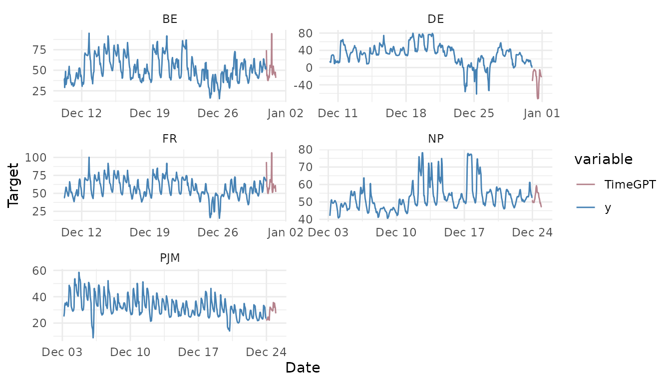
#> 6 BE 2016-12-31 05:00:00 51.497254. Plot TimeGPT forecast
nixtlar includes a function to plot the historical data
and any output from nixtla_client_forecast,
nixtla_client_historic,
nixtla_client_anomaly_detection and
nixtla_client_cross_validation. If you have long series,
you can use max_insample_length to only plot the last N
historical values (the forecast will always be plotted in full).
nixtla_client_plot(df_exo_vars, fcst_exo_vars, max_insample_length = 500)