1. Long-horizon forecasting
In some cases, it is necessary to forecast long horizons. Here “long horizons” refer to predictions that exceed more than two seasonal periods. For example, this would mean forecasting more than 48 hours ahead for hourly data or more than 7 days for daily data. The specific definition of “long horizon” varies depending on the data frequency.
There is a specialized TimeGPT model designed for
long-horizon forecasting, which is trained to predict far into the
future, where the uncertainty increases as the forecast extends further.
Here we will explain how to use the long horizon model of
TimeGPT via nixtlar.
This vignette assumes you have already set up your API key. If you haven’t done this, please read the Get Started vignette first.
2. Load data
For this vignette, we’ll use the electricity consumption dataset that
is included in nixtlar, which contains the hourly prices of
five different electricity markets.
df <- nixtlar::electricity
head(df)
#>   unique_id                  ds     y
#> 1        BE 2016-10-22 00:00:00 70.00
#> 2        BE 2016-10-22 01:00:00 37.10
#> 3        BE 2016-10-22 02:00:00 37.10
#> 4        BE 2016-10-22 03:00:00 44.75
#> 5        BE 2016-10-22 04:00:00 37.10
#> 6        BE 2016-10-22 05:00:00 35.61
For every unique_id, we’ll try to predict the last 96
hours. Hence, we will first separate the data into training and test
sets.
test <- df |>
  dplyr::group_by(unique_id) |>
  dplyr::slice_tail(n = 96) |>
  dplyr::ungroup()

train <- df[df$ds %in% setdiff(df$ds, test$ds), ]
3. Forecast with a long-horizon
To use the long-horizon model of TimeGPT, set the
model argument to timegpt-1-long-horizon.
fcst_long_horizon <- nixtlar::nixtla_client_forecast(train, h=96, model="timegpt-1-long-horizon")
#> Frequency chosen: h
head(fcst_long_horizon)
#>   unique_id                  ds  TimeGPT
#> 1        BE 2016-12-27 00:00:00 42.73280
#> 2        BE 2016-12-27 01:00:00 38.03184
#> 3        BE 2016-12-27 02:00:00 35.11706
#> 4        BE 2016-12-27 03:00:00 34.53464
#> 5        BE 2016-12-27 04:00:00 34.11326
#> 6        BE 2016-12-27 05:00:00 38.36180
4. Plot the long-horizon forecast
nixtlar includes a function to plot the historical data
and any output from nixtlar::nixtla_client_forecast,
nixtlar::nixtla_client_historic,
nixtlar::nixtla_client_detect_anomalies and
nixtlar::nixtla_client_cross_validation. If you have long
series, you can use max_insample_length to only plot the
last N historical values (the forecast will always be plotted in
full).
nixtlar::nixtla_client_plot(train, fcst_long_horizon, max_insample_length = 200)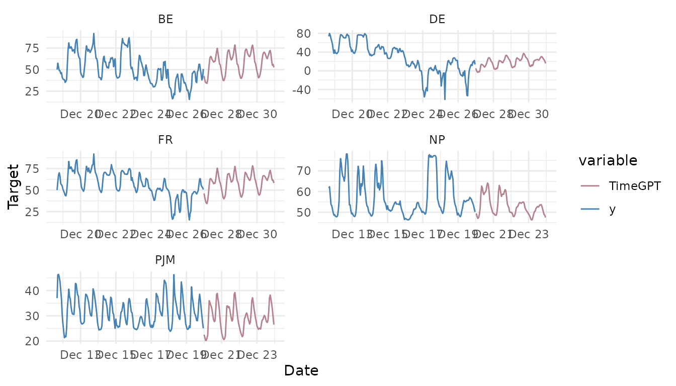
5. Evaluate the long-horizon model
To evaluate the long-horizon forecast, we will generate the same
forecast with the default model of TimeGPT, which is
timegpt-1, and then we will compute and compare the Mean Absolute
Error (MAE) of the two models.
fcst <- nixtlar::nixtla_client_forecast(train, h=96)
#> Frequency chosen: h
#> The specified horizon h exceeds the model horizon. This may lead to less accurate forecasts. Please consider using a smaller horizon.
head(fcst)
#>   unique_id                  ds  TimeGPT
#> 1        BE 2016-12-27 00:00:00 45.21921
#> 2        BE 2016-12-27 01:00:00 42.56666
#> 3        BE 2016-12-27 02:00:00 41.55990
#> 4        BE 2016-12-27 03:00:00 39.12502
#> 5        BE 2016-12-27 04:00:00 36.47087
#> 6        BE 2016-12-27 05:00:00 37.22281
We will rename the TimeGPT long-horizon model to merge
it with the default TimeGPT model. After that, we will
combine them with the actual values from the test set and compute the
MAE. Note that in the output of the nixtla_client_forecast
function, the ds column contains dates. This is because
nixtla_client_plot uses the dates for plotting. However, to
merge the actual values, we will convert the dates to characters.
names(fcst_long_horizon)[which(names(fcst_long_horizon) == "TimeGPT")] <- "TimeGPT-long-horizon"

res <- merge(fcst, fcst_long_horizon) # merge TimeGPT and TimeGPT-long-horizon
res$ds <- as.character(res$ds)

res <- merge(test, res) # merge with actual values
head(res)
#>   unique_id                  ds     y  TimeGPT TimeGPT-long-horizon
#> 1        BE 2016-12-27 01:00:00 38.33 42.56666             38.03184
#> 2        BE 2016-12-27 02:00:00 41.04 41.55990             35.11706
#> 3        BE 2016-12-27 03:00:00 34.62 39.12502             34.53464
#> 4        BE 2016-12-27 04:00:00 29.69 36.47087             34.11326
#> 5        BE 2016-12-27 05:00:00 28.35 37.22281             38.36180
#> 6        BE 2016-12-27 06:00:00 30.99 42.28119             47.14175
print(paste0("MAE TimeGPT: ", mean(abs(res$y-res$TimeGPT))))
#> [1] "MAE TimeGPT: 8.89928802286956"
print(paste0("MAE TimeGPT long-horizon: ", mean(abs(res$y-res$`TimeGPT-long-horizon`))))
#> [1] "MAE TimeGPT long-horizon: 7.09790721521739"
As we can see, the long-horizon version of TimeGPT
produced a model with a lower MAE than the default TimeGPT
model.