1. Uncertainty quantification via quantiles
For uncertainty quantification, TimeGPT can generate
both prediction intervals and quantiles, offering a measure of the range
of potential outcomes rather than just a single point forecast. In
real-life scenarios, forecasting often requires considering multiple
alternatives, not just one prediction. This vignette will explain how to
use quantiles with TimeGPT via the nixtlar
package.
Quantiles represent the cumulative proportion of the forecast
distribution. For instance, the 90th quantile is the value below which
90% of the data points are expected to fall. Notably, the 50th quantile
corresponds to the median forecast value provided by
TimeGPT. The quantiles are produced using conformal
prediction, a framework for creating distribution-free uncertainty
intervals for predictive models.
This vignette assumes you have already set up your API key. If you haven’t done this, please read the Get Started vignette first.
2. Load data
For this vignette, we will use the electricity consumption dataset
that is included in nixtlar, which contains the hourly
prices of five different electricity markets.
df <- nixtlar::electricity
head(df)
#>   unique_id                  ds     y
#> 1        BE 2016-10-22 00:00:00 70.00
#> 2        BE 2016-10-22 01:00:00 37.10
#> 3        BE 2016-10-22 02:00:00 37.10
#> 4        BE 2016-10-22 03:00:00 44.75
#> 5        BE 2016-10-22 04:00:00 37.10
#> 6        BE 2016-10-22 05:00:00 35.61
3. Forecast with quantiles
TimeGPT can generate quantiles when using the following
functions:
- nixtlar::nixtla_client_forecast()
- nixtlar::nixtla_client_historic()
- nixtlar::nixtla_client_cross_validation()
For any of these functions, simply set the quantiles
argument to the desired values as a vector. Keep in mind that quantiles
should all be numbers between 0 and 1. You can use either
quantiles or level for uncertainty
quantification, but not both.
fcst <- nixtla_client_forecast(df, h = 8, quantiles = c(0.1, 0.2, 0.3, 0.4, 0.5, 0.6, 0.7, 0.8, 0.9))
#> Frequency chosen: h
head(fcst)
#> unique_id ds TimeGPT TimeGPT-q-10 TimeGPT-q-20 TimeGPT-q-30
#> 1 BE 2016-12-31 00:00:00 45.19067 35.50871 38.47807 40.71672
#> 2 BE 2016-12-31 01:00:00 43.24491 35.37606 37.77021 39.32019
#> 3 BE 2016-12-31 02:00:00 41.95889 35.34064 37.21904 39.44587
#> 4 BE 2016-12-31 03:00:00 39.79668 32.32713 34.98742 35.96046
#> 5 BE 2016-12-31 04:00:00 39.20456 30.99962 32.74742 34.72213
#> 6 BE 2016-12-31 05:00:00 40.10912 32.43535 34.24889 35.10847
#> TimeGPT-q-40 TimeGPT-q-50 TimeGPT-q-60 TimeGPT-q-70 TimeGPT-q-80 TimeGPT-q-90
#> 1 43.92536 45.19067 46.45599 49.66462 51.90328 54.87264
#> 2 42.58577 43.24491 43.90405 47.16964 48.71962 51.11376
#> 3 40.85597 41.95889 43.06182 44.47191 46.69875 48.57715
#> 4 37.46490 39.79668 42.12846 43.63290 44.60593 47.26623
#> 5 36.01357 39.20456 42.39555 43.68699 45.66169 47.40950
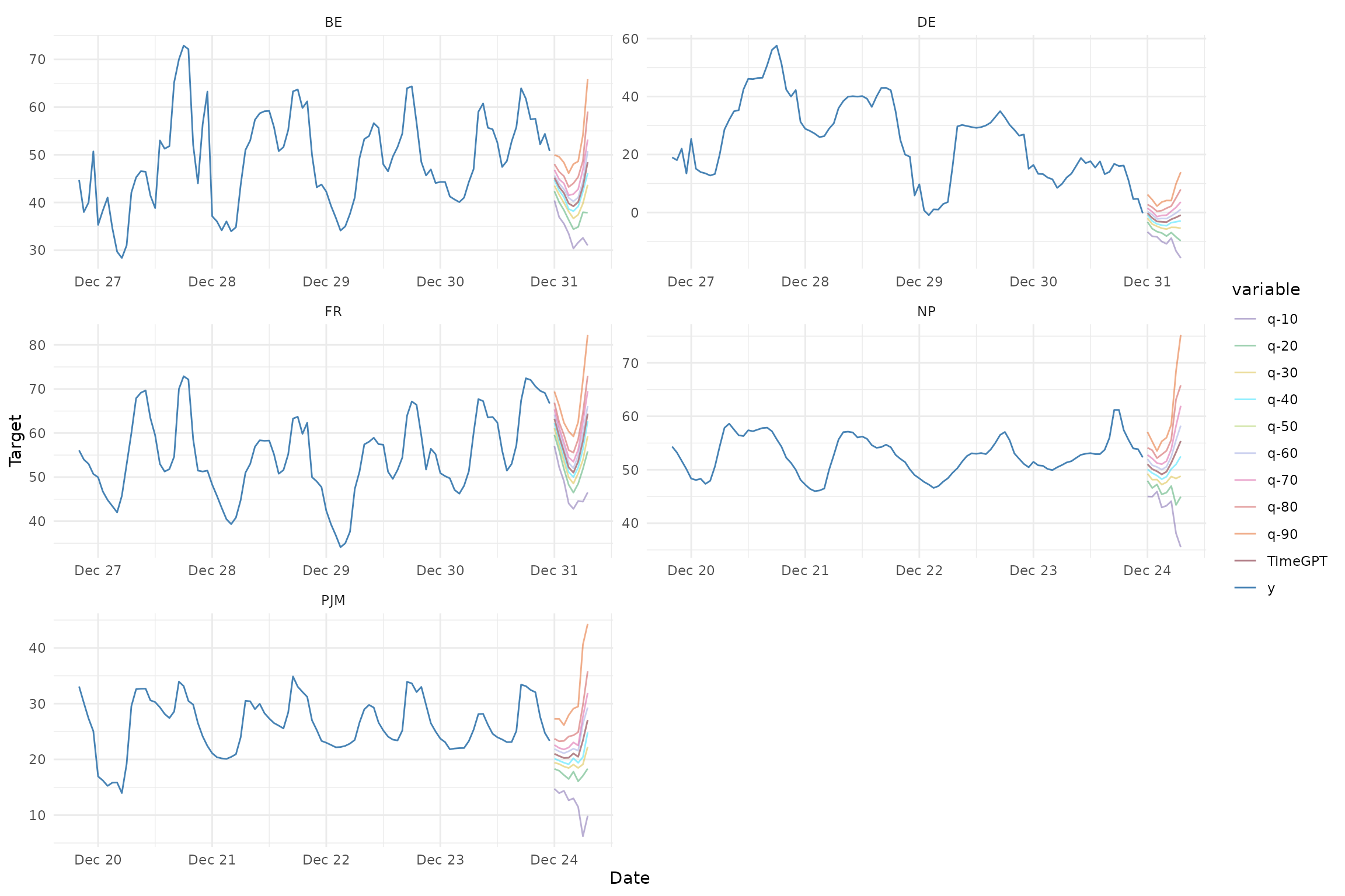
#> 6 38.76706 40.10912 41.45117 45.10976 45.96934 47.782884. Plot quantiles
nixtlar includes a function to plot the historical data
and any output from nixtlar::nixtla_client_forecast,
nixtlar::nixtla_client_historic,
nixtlar::nixtla_client_detect_anomalies and
nixtlar::nixtla_client_cross_validation. If you have long
series, you can use max_insample_length to only plot the
last N historical values (the forecast will always be plotted in
full).
When available, nixtlar::nixtla_client_plot will
automatically plot the quantiles.
nixtla_client_plot(df, fcst, max_insample_length = 100)