Prediction Intervals • nixtlar

library(nixtlar)

1. Uncertainty quantification via prediction intervals

For uncertainty quantification, TimeGPT can generate both prediction intervals and quantiles, offering a measure of the range of potential outcomes rather than just a single point forecast. In real-life scenarios, forecasting often requires considering multiple alternatives, not just one prediction. This vignette will explain how to use prediction intervals with TimeGPT via the nixtlar package.

A prediction interval is a range of values that the forecast can take with a given probability, often referred to as the confidence level. Hence, a 95% prediction interval should contain a range of values that includes the actual future value with a probability of 95%. Prediction intervals are part of probabilistic forecasting, which, unlike point forecasting, aims to generate the full forecast distribution instead of just the mean or the median of that distribution.

This vignette assumes you have already set up your API key. If you haven’t done this, please read the Get Started vignette first.

2. Load data

For this vignette, we’ll use the electricity consumption dataset that is included in nixtlar, which contains the hourly prices of five different electricity markets.

df <- nixtlar::electricity
head(df)
#>   unique_id                  ds     y
#> 1        BE 2016-10-22 00:00:00 70.00
#> 2        BE 2016-10-22 01:00:00 37.10
#> 3        BE 2016-10-22 02:00:00 37.10
#> 4        BE 2016-10-22 03:00:00 44.75
#> 5        BE 2016-10-22 04:00:00 37.10
#> 6        BE 2016-10-22 05:00:00 35.61

3. Forecast with prediction intervals

TimeGPT can generate prediction intervals when using the following functions:

- nixtlar::nixtla_client_forecast()
- nixtlar::nixtla_client_historic() 
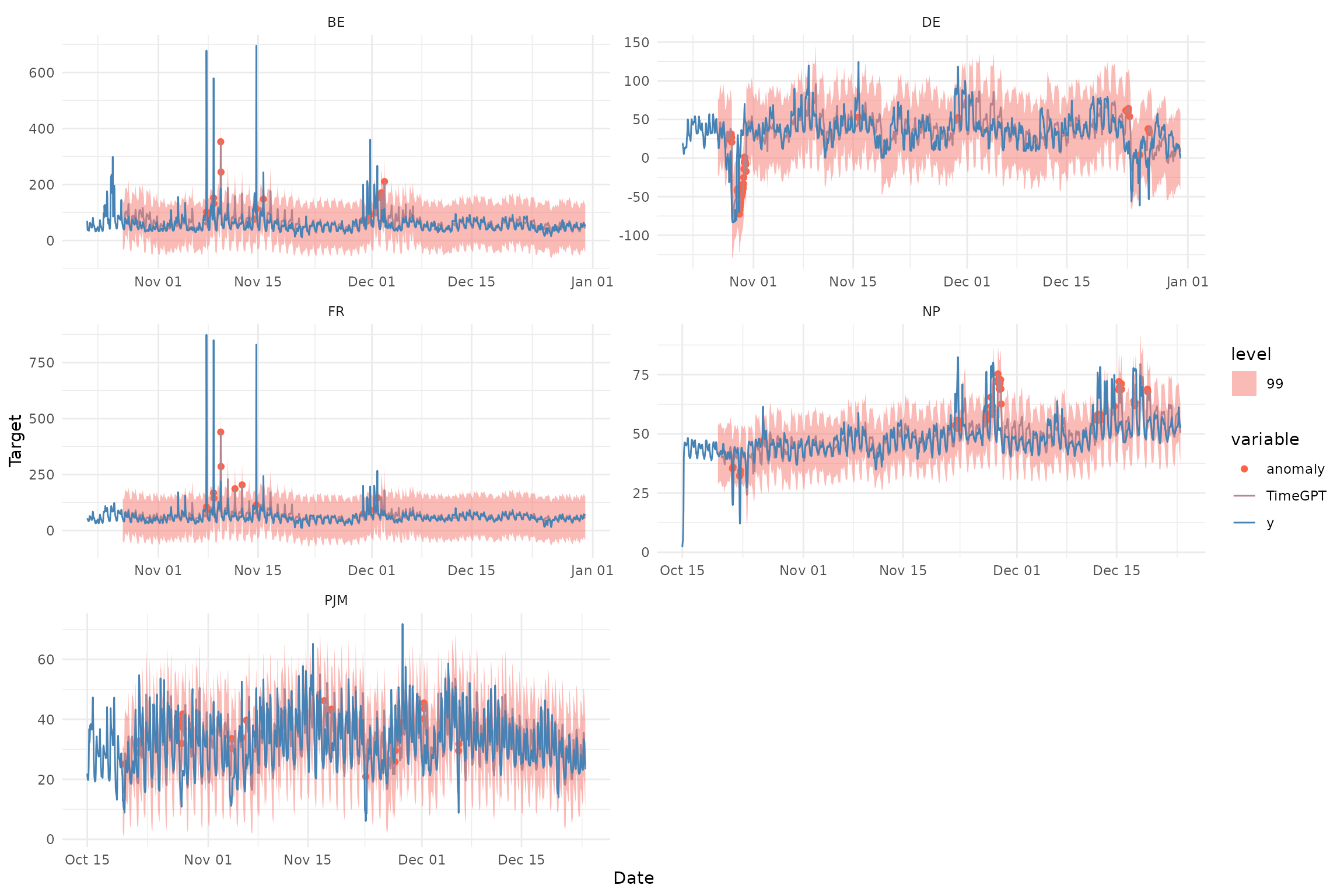
- nixtlar::nixtla_client_detect_anomalies()
- nixtlar::nixtla_client_cross_validation()

For any of these functions, simply set the level argument to the desired confidence level for the prediction intervals. Keep in mind that level should be a vector with numbers between 0 and 100. You can use either quantiles or level for uncertainty quantification, but not both.

fcst <- nixtla_client_forecast(df, h = 8, level=c(80,95))
#> Frequency chosen: h
head(fcst)
#>   unique_id                  ds  TimeGPT TimeGPT-lo-95 TimeGPT-lo-80
#> 1        BE 2016-12-31 00:00:00 45.19045      30.49691      35.50842
#> 2        BE 2016-12-31 01:00:00 43.24445      28.96423      35.37463
#> 3        BE 2016-12-31 02:00:00 41.95839      27.06667      35.34079
#> 4        BE 2016-12-31 03:00:00 39.79649      27.96751      32.32625
#> 5        BE 2016-12-31 04:00:00 39.20454      24.66072      30.99895
#> 6        BE 2016-12-31 05:00:00 40.10878      23.05056      32.43504
#>   TimeGPT-hi-80 TimeGPT-hi-95
#> 1      54.87248      59.88399
#> 2      51.11427      57.52467
#> 3      48.57599      56.85011
#> 4      47.26672      51.62546
#> 5      47.41012      53.74836
#> 6      47.78252      57.16700

Note that the level argument in the nixtlar::nixtla_client_detect_anomalies() function uses only the maximum value when there are multiple values. Hence, setting level=c(90,95,99), for example, is equivalent to setting level=c(99), which is the default value.

anomalies <- nixtla_client_detect_anomalies(df) # level=c(90,95,99)
#> Frequency chosen: h
head(anomalies) # only the 99% confidence level is used 
#>   unique_id                  ds     y anomaly  TimeGPT TimeGPT-lo-99
#> 1        BE 2016-10-27 00:00:00 52.58   FALSE 56.07623     -28.58337
#> 2        BE 2016-10-27 01:00:00 44.86   FALSE 52.41973     -32.23986
#> 3        BE 2016-10-27 02:00:00 42.31   FALSE 52.81474     -31.84486
#> 4        BE 2016-10-27 03:00:00 39.66   FALSE 52.59026     -32.06934
#> 5        BE 2016-10-27 04:00:00 38.98   FALSE 52.67297     -31.98662
#> 6        BE 2016-10-27 05:00:00 42.31   FALSE 54.10659     -30.55301
#>   TimeGPT-hi-99
#> 1      140.7358
#> 2      137.0793
#> 3      137.4743
#> 4      137.2499
#> 5      137.3326
#> 6      138.7662

4. Plot prediction intervals

nixtlar includes a function to plot the historical data and any output from nixtlar::nixtla_client_forecast, nixtlar::nixtla_client_historic, nixtlar::nixtla_client_detect_anomalies and nixtlar::nixtla_client_cross_validation. If you have long series, you can use max_insample_length to only plot the last N historical values (the forecast will always be plotted in full).

When available, nixtlar::nixtla_client_plot will automatically plot the prediction intervals.

nixtla_client_plot(df, fcst, max_insample_length = 100)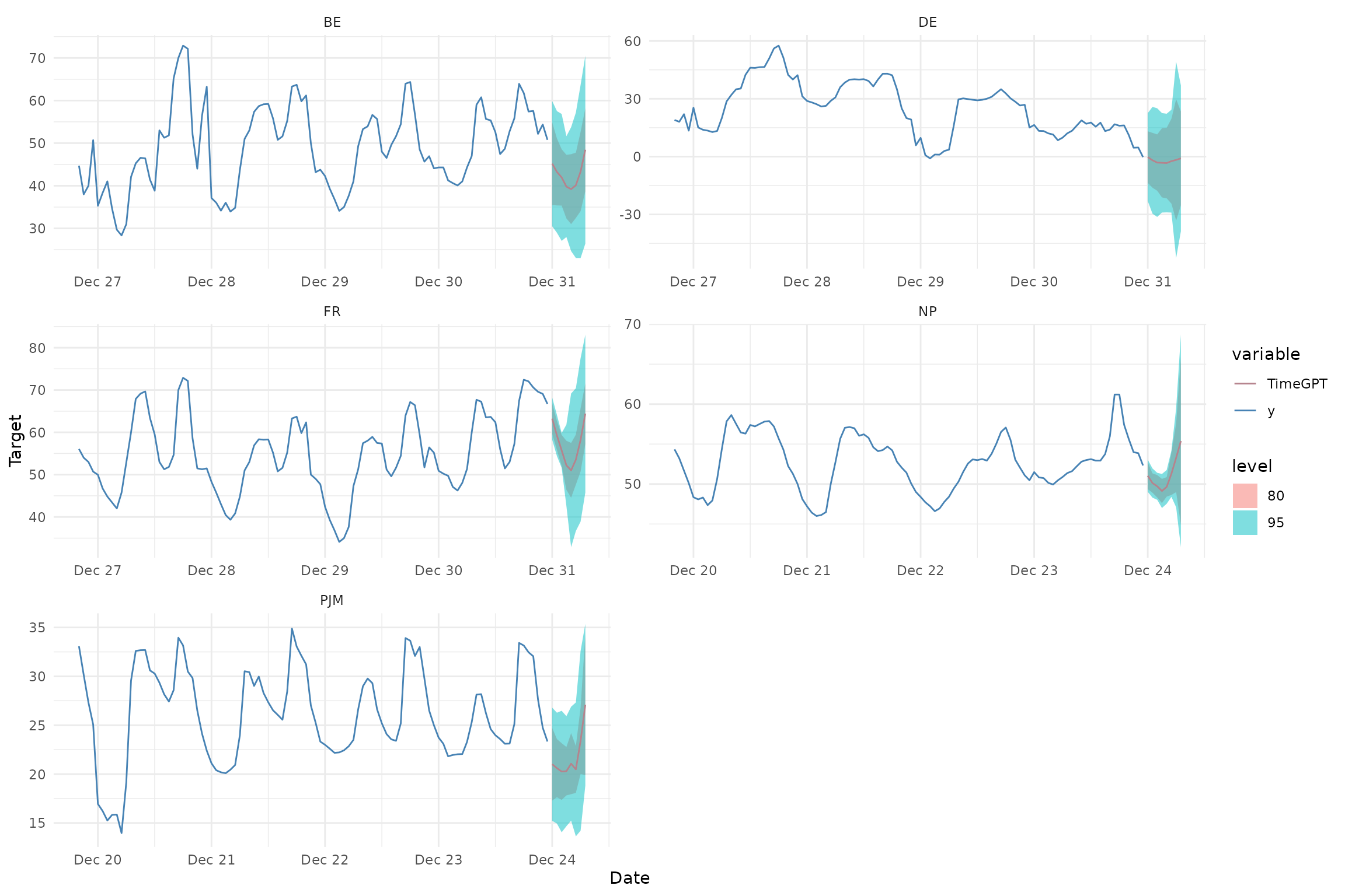

nixtlar::nixtla_client_plot(df, anomalies, plot_anomalies = TRUE)