Get Started

library(nixtlar)

nixtlar provides an R interface to Nixtla’s TimeGPT, a generative pre-trained forecasting model for time series data. TimeGPT is the first foundation model capable of producing accurate forecasts for new time series not seen during training, using only its historical values as inputs. TimeGPT can also be used for other time series related tasks, such as anomaly detection and cross-validation. Here we explain how to get started with TimeGPT in R and give a quick overview of the main features of nixtlar.

1. Setting up your API key

First, you need to set up your API key. An API key is a string of characters that allows you to authenticate your requests when using TimeGPT via nixtlar. This API key needs to be provided by Nixtla, so if you don’t have one, please request one here.

When using nixtlar, there are two ways of setting up your API key:

a. Using the `nixtla_client_setup` function

nixtlar has a function to easily set up your API key for your current R session. Simply call

nixtla_client_setup(api_key = "Your API key here")

Keep in mind that if you close your R session or you re-start it, then you’ll need to set up your API key again.

When using Azure, you also need to add the base_ur parameter to the nixtla_client_setup function.

nixtla_client_setup(
  base_url = "Base ULR",
  api_key = "Your API key here"
)

b. Using an environment variable

For a more persistent method that can be used across different projects, set up your API key as environment variable. To do this, first load the usethis package.

library(usethis)
usethis::edit_r_environ()

This will open your .Reviron file. Place your API key here and named it NIXTLA_API_KEY.

# Inside the .Renviron file 
NIXTLA_API_KEY="Your API key here"

You’ll need to restart R for changes to take effect. Keep in mind that modifying the .Renviron file affects all of your R sessions, so if you’re not comfortable with this, use the nixtla_client_setup function instead.

If you are using Azure, you also need to specify the NIXTLA_BASE_URL.

# Inside the .Renviron file 
NIXTLA_BASE_URL="Base URL"
NIXTLA_API_KEY="Your API key here"

For details on how to set up your API key, check out the Setting Up Your API Key vignette. To learn more about how to use Azure, please refer to the TimeGEN-1 Quickstart (Azure).

Validate your API key

If you want to validate your API key, call nixtla_validate_api_key.

nixtla_validate_api_key()

You don’t need to validate your API key every time you set it up, only when you want to check if it’s valid. The nixtla_validate_api_key will return TRUE if you API key is valid, and FALSE otherwise.

2. Generate TimeGPT forecast

Once your API key has been set up, you’re ready to use TimeGPT. Here we’ll show you how this is done using a dataset that contains prices of different electricity markets.

df <- nixtlar::electricity
head(df)
#>   unique_id                  ds     y
#> 1        BE 2016-10-22 00:00:00 70.00
#> 2        BE 2016-10-22 01:00:00 37.10
#> 3        BE 2016-10-22 02:00:00 37.10
#> 4        BE 2016-10-22 03:00:00 44.75
#> 5        BE 2016-10-22 04:00:00 37.10
#> 6        BE 2016-10-22 05:00:00 35.61

To generate a forecast for this dataset, use nixtla_client_forecast. Default names for the time and the target columns are ds and y. If your time and target columns have different names, specify them with time_col and target_col. Since it has multiple ids (one for every electricity market), you’ll need to specify the name of the column that contains the ids, which in this case is unique_id. To do this, simply use id_col="unique_id". You can also choose confidence levels (0-100) for prediction intervals with level.

nixtla_client_fcst <- nixtla_client_forecast(df, h = 8, level = c(80,95))
#> Frequency chosen: h
head(nixtla_client_fcst)
#>   unique_id                  ds  TimeGPT TimeGPT-lo-95 TimeGPT-lo-80
#> 1        BE 2016-12-31 00:00:00 45.19045      30.49691      35.50842
#> 2        BE 2016-12-31 01:00:00 43.24445      28.96423      35.37463
#> 3        BE 2016-12-31 02:00:00 41.95839      27.06667      35.34079
#> 4        BE 2016-12-31 03:00:00 39.79649      27.96751      32.32625
#> 5        BE 2016-12-31 04:00:00 39.20454      24.66072      30.99895
#> 6        BE 2016-12-31 05:00:00 40.10878      23.05056      32.43504
#>   TimeGPT-hi-80 TimeGPT-hi-95
#> 1      54.87248      59.88399
#> 2      51.11427      57.52467
#> 3      48.57599      56.85011
#> 4      47.26672      51.62546
#> 5      47.41012      53.74836
#> 6      47.78252      57.16700

3. Plot TimeGPT forecast

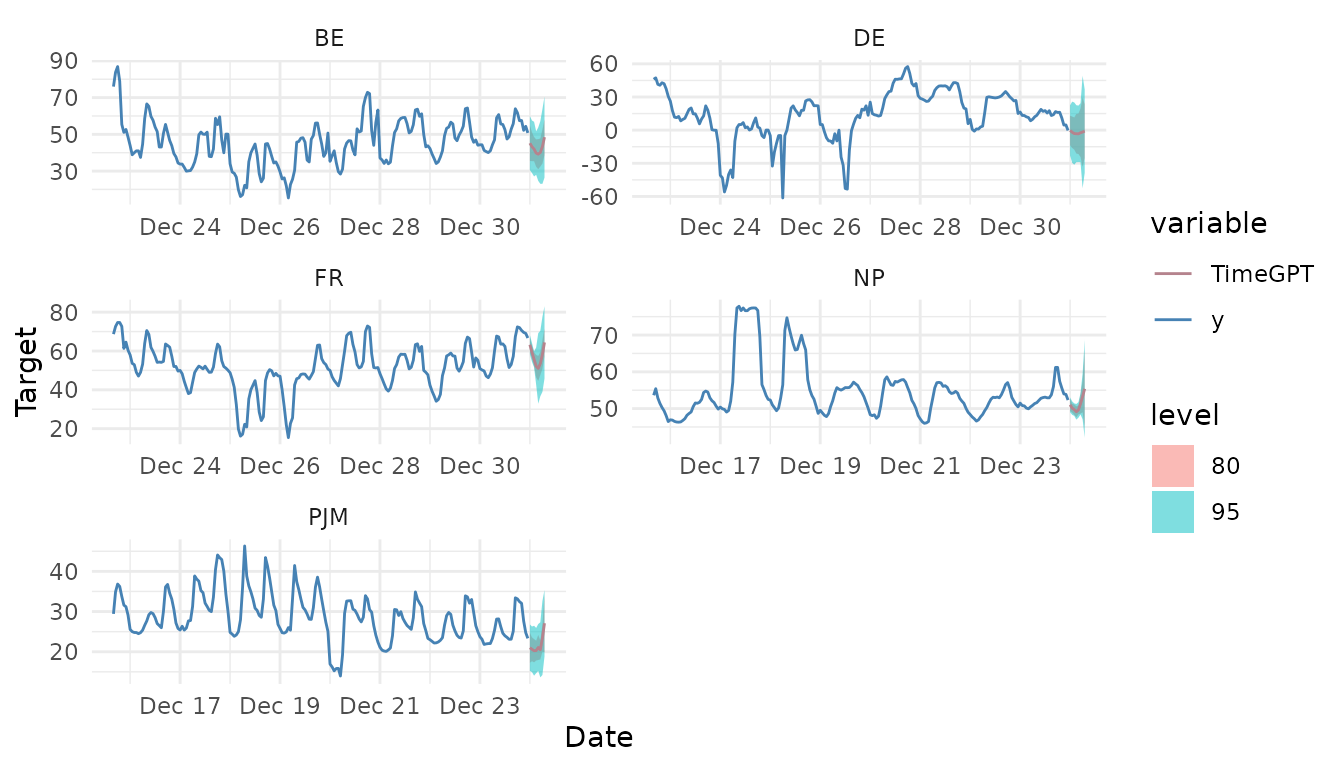
nixtlar includes a function to plot the historical data and any output from nixtla_client_forecast, nixtla_client_historic, nixtla_client_anomaly_detection and nixtla_client_cross_validation. If you have long series, you can use max_insample_length to only plot the last N historical values (the forecast will always be plotted in full).