1. Anomaly detection
Anomaly detection plays a crucial role in time series analysis and forecasting. Anomalies, also known as outliers, are unusual observations that don’t follow the expected time series patterns. They can be caused by a variety of factors, including errors in the data collection process, unexpected events, or sudden changes in the patterns of the time series. Anomalies can provide critical information about a system, like a potential problem or malfunction. After identifying them, it is important to understand what caused them, and then decide whether to remove, replace, or keep them.
TimeGPT has a method for detecting anomalies, and users
can call it from nixtlar. This vignette will explain how to
do this. It assumes you have already set up your API key. If you haven’t
done this, please read the Get
Started vignette first.
2. Load data
For this vignette, we’ll use the electricity consumption dataset that
is included in nixtlar, which contains the hourly prices of
five different electricity markets.
df <- nixtlar::electricity
head(df)
#>   unique_id                  ds     y
#> 1        BE 2016-10-22 00:00:00 70.00
#> 2        BE 2016-10-22 01:00:00 37.10
#> 3        BE 2016-10-22 02:00:00 37.10
#> 4        BE 2016-10-22 03:00:00 44.75
#> 5        BE 2016-10-22 04:00:00 37.10
#> 6        BE 2016-10-22 05:00:00 35.61
3. Detect Anomalies
To detect anomalies, use
nixtlar::nixtla_client_detect_anomalies, which requires the
following parameter:
-
df: The time series data, provided as a data frame,
tibble, or tsibble. It must include at least two columns: one for the
timestamps and one for the observations. The default names for these
columns are
dsandy. If your column names are different, specify them withtime_colandtarget_col, respectively. If you are working with multiple series, you must also include a column with unique identifiers. The default name for this column isunique_id; if different, specify it withid_col.
nixtla_client_anomalies <- nixtlar::nixtla_client_detect_anomalies(df)
#> Frequency chosen: h
head(nixtla_client_anomalies)
#>   unique_id                  ds     y anomaly  TimeGPT TimeGPT-lo-99
#> 1        BE 2016-10-27 00:00:00 52.58   FALSE 56.07206     -28.58840
#> 2        BE 2016-10-27 01:00:00 44.86   FALSE 52.41392     -32.24654
#> 3        BE 2016-10-27 02:00:00 42.31   FALSE 52.80694     -31.85352
#> 4        BE 2016-10-27 03:00:00 39.66   FALSE 52.58330     -32.07716
#> 5        BE 2016-10-27 04:00:00 38.98   FALSE 52.66963     -31.99083
#> 6        BE 2016-10-27 05:00:00 42.31   FALSE 54.10218     -30.55829
#>   TimeGPT-hi-99
#> 1      140.7325
#> 2      137.0744
#> 3      137.4674
#> 4      137.2438
#> 5      137.3301
#> 6      138.7626
The anomaly_detection method from TimeGPT
evaluates each observation and uses a prediction interval to determine
if it is an anomaly or not. By default,
nixtlar::nixtla_client_detect_anomalies uses a 99%
prediction interval. Observations that fall outside this interval will
be considered anomalies and will have a value of True in
the anomaly column (False otherwise). To
change the prediction interval, for example to 95%, use the argument
level=c(95). Keep in mind that multiple levels are not
allowed, so when given several values,
nixtlar::nixtla_client_detect_anomalies will use the
maximum.
4. Plot anomalies
nixtlar includes a function to plot the historical data
and any output from nixtlar::nixtla_client_forecast,
nixtlar::nixtla_client_historic,
nixtlar::nixtla_client_detect_anomalies and
nixtlar::nixtla_client_cross_validation. If you have long
series, you can use max_insample_length to only plot the
last N historical values (the forecast will always be plotted in
full).
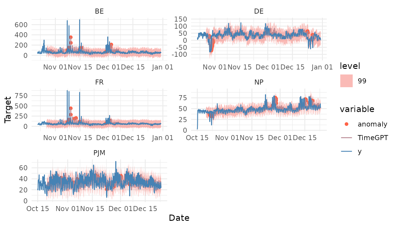
When using nixtlar::nixtla_client_plot with the output
of nixtlar::nixtla_client_detect_anomalies, set
plot_anomalies=TRUE to plot the anomalies.
nixtlar::nixtla_client_plot(df, nixtla_client_anomalies, plot_anomalies = TRUE)